Skin Conductance Response
Data Cleaning
# Load data
load(file = "./data/Single_Trial_Data.rda")


# Before trial exclusion, create variable indicating color of fixation cross (needed for control analysis)
# Trial after each fast hit starts with white fixation cross; all other trials with red cross
single_trial_data <- single_trial_data %>%
  mutate(
    fixation_cross_white = (lag(gng_response_type) == "FH")
  )


# First trial of each block also starts with white fixation cross
single_trial_data[single_trial_data$trial == 1   | single_trial_data$trial == 29  |
                  single_trial_data$trial == 101 | single_trial_data$trial == 173 |
                  single_trial_data$trial == 201 | single_trial_data$trial == 273 |
                  single_trial_data$trial == 345 | single_trial_data$trial == 373 |
                  single_trial_data$trial == 445,]$fixation_cross_white <- TRUE


# For SCR analysis, exclude exclude inhibited gng responses, missing responses, responses with wrong key, trials with
# incorrect word categorization, RT outliers, and trials that were followed or preceded by trials with incorrect responses
single_trial_data_scr <- single_trial_data %>%
  dplyr::filter(
      gng_response_type != "IR" &
      gng_response_type != "miss" &
      gng_response_type != "wrong_key" &
      word_accuracy     != "incorrect" &
      word_accuracy     != "miss" &
      word_accuracy     != "wrong_key" &
      (is.na(gng_rt_invalid)  | gng_rt_invalid  == FALSE) &
      (is.na(word_rt_outlier) | word_rt_outlier == FALSE) &
      trial_followed_or_preceded_by_any_incorr_resp == FALSE &
      !is.na(iscr_gng_resp)
  ) # (7139 of 15480 trials left)


# Calculate standardized SCR and standardized square root transformed SCR
single_trial_data_scr <- single_trial_data_scr %>%
  dplyr::group_by(participant_id) %>%
  dplyr::mutate(
      iscr_gng_resp_sqrt   = sqrt(iscr_gng_resp),
      iscr_gng_resp_z      = scale(iscr_gng_resp, center = TRUE, scale = TRUE),
      iscr_gng_resp_sqrt_z = scale(sqrt(iscr_gng_resp), center = TRUE, scale = TRUE)
    ) %>%
  dplyr::ungroup()


# Make categorical variables factors
single_trial_data_scr$gng_response_type     <- factor(single_trial_data_scr$gng_response_type, levels = c("SH", "FH", "FA"))
single_trial_data_scr$word_valence          <- factor(single_trial_data_scr$word_valence)
single_trial_data_scr$participant_id        <- factor(single_trial_data_scr$participant_id)
single_trial_data_scr$word                  <- factor(single_trial_data_scr$word)
single_trial_data_scr$fixation_cross_white  <- factor(single_trial_data_scr$fixation_cross_white, levels = c(TRUE, FALSE))
Trials were excluded from all analyses if RT in the go/no-go task was shorter than 100 ms or longer than 700 ms, or if the word categorization RT was more than three median absolute deviations (Leys et al., 2013) above or below a participant’s median RT computed per condition. We further discarded trials in which responses in the go/no-go task were missing or performed with one of the word categorization keys. For analyses containing SCR as dependent or independent variable, we included only trials with correct word categorization that were neither followed nor preceded by trials in which incorrect responses were made. Moreover, only slow hit, fast hit, and false alarm trials were included in SCR analyses. For details on the percentage of excluded trials, please see section “Data Cleaning” in the tab “Word Categorization Task”.
Descriptive Statistics
Means and CIs
This table corresponds to Table S9 in the supplemental material.
# Calculate descriptive statistics for standardized SCR per condition
descriptive_statistics_scr_z <- summarySEwithinO(
  data          = single_trial_data_scr,
  measurevar    = "iscr_gng_resp_z",
  withinvars    = "gng_response_type",
  idvar         = "participant_id",
  conf.interval = .95
) %>%
  # Format confidence interval column
  dplyr::mutate(
    ci_scr = paste0("[", round(iscr_gng_resp_z - ci, digits = 2),
                    ", ", round(iscr_gng_resp_z + ci, digits = 2), "]")
  ) %>%
  # Round numeric values to two decimals
  dplyr::mutate_if(is.numeric, round, digits = 2) %>%
  # Select columns to be displayed
  dplyr::select(c("gng_response_type", "iscr_gng_resp_z", "ci_scr", "ci"))


# Display descriptive statistics for standardized SCR (and rearrange order of rows)
my_table_template(descriptive_statistics_scr_z[c(3, 2, 1), c(1:3)],
  caption = "Standardized SCR (µS)",
  col_names = c("Response type", "M", "95% CI"),
  footnote_config = c(general = "Confidence intervals are adjusted for within-participant designs as described by Morey (2008).")
)| Response type | M | 95% CI |
|---|---|---|
| SH | -0.07 | [-0.11, -0.03] |
| FH | -0.02 | [-0.06, 0.03] |
| FA | 0.32 | [0.22, 0.41] |
| Note: | ||
| Confidence intervals are adjusted for within-participant designs as described by Morey (2008). |
Plot
This figure corresponds to Figure 3 in the manuscript.
# Create plot standardized SCR
plot_scr <- ggplot(descriptive_statistics_scr_z,
                  aes(x = gng_response_type, y = iscr_gng_resp_z)) +
  geom_bar(stat = "identity", position = position_dodge(), colour = "black", size = 0.25, fill = "#8ea6b4") +
  geom_errorbar(aes(ymax = iscr_gng_resp_z + ci, ymin = iscr_gng_resp_z - ci),
                position = position_dodge(width = 0.9), width = 0.2, size = 0.3) +
  my_figure_theme +
  labs(x = "Response Type", y = "Standardized SCR (µS)") +
  coord_cartesian(ylim = c(-0.2,0.5)) +
  scale_y_continuous(breaks = seq(-0.2, 0.5, 0.1), expand = c(0,0)) +
  geom_hline(yintercept = 0, size = 0.25) +
  geom_signif(
    y_position = c(0.47,0.43), xmin = c(1,2), xmax = c(3,3),
    annotation = c("***","**"), tip_length = 0.01, vjust = 0.5, textsize = 4, size = 0.3
  )


# Save plot
# ggsave("figure_scr.tiff",width = 10, height = 7.5 , units = "cm", dpi=600, compression = "lzw")


# Display plot
plot_scr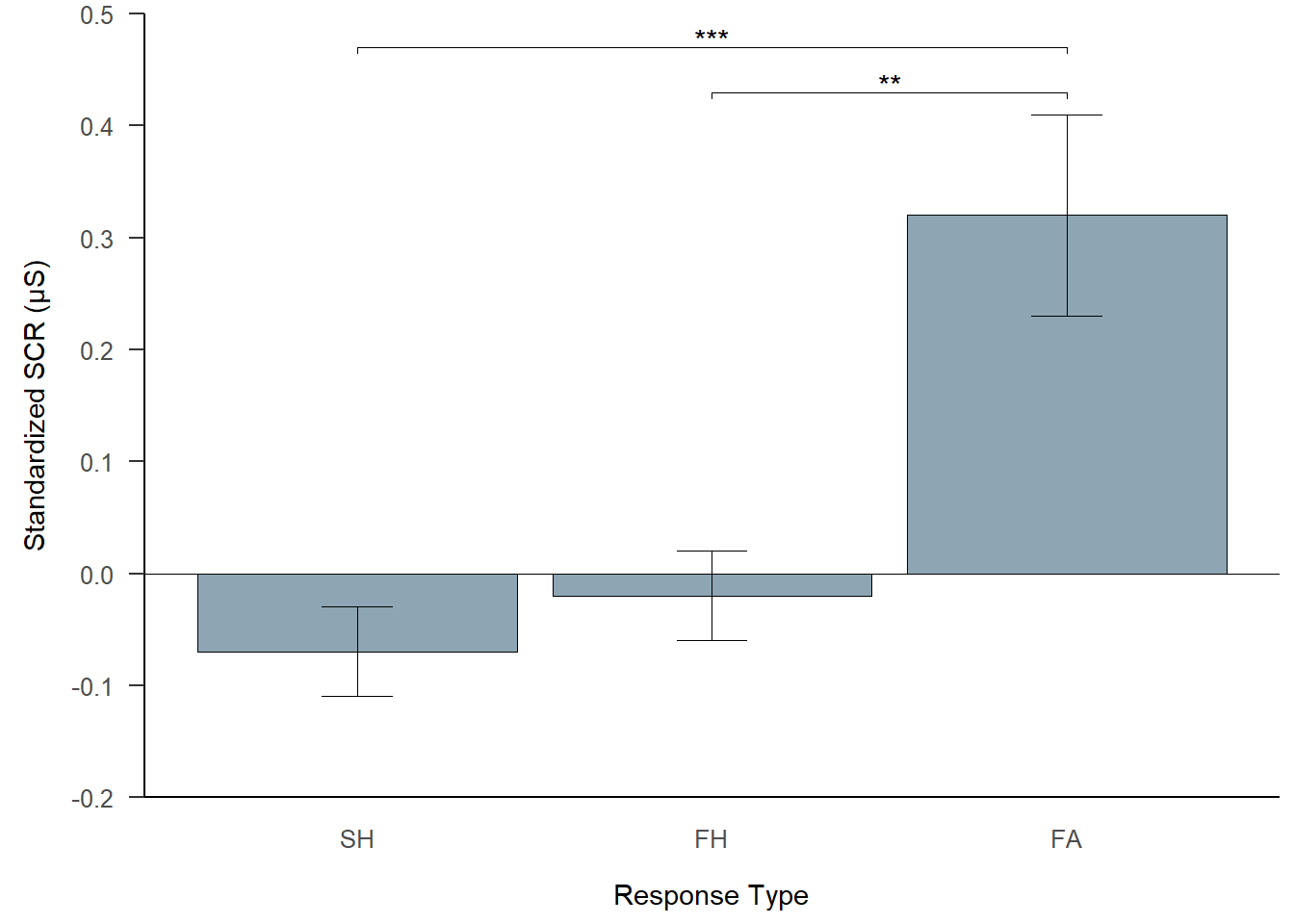
Note. Standardized SCR is shown as a function of response type in the go/no-go task. Error bars represent 95% confidence intervals adjusted for within-participant designs as described by Morey (2008). Asterisks refer to significant differences based on linear mixed-effects model analysis.
Physiological nonresponders
Participants exhibiting no measurable SCR (i.e., ISCR scores of zero) in more than 75% of all trials were classified as physiological nonresponders. All participants were below this threshold, so no participants were excluded from SCR analyses.
# Calculate percentage of zero responses (based on all trials)
zero_responses <- single_trial_data[!is.na(single_trial_data$iscr_gng_resp), ] %>%
  dplyr::group_by(participant_id) %>%
  dplyr::summarize(
    percentage_zero_responses = length(participant_id[iscr_gng_resp == 0]) / length(participant_id) * 100
  ) %>%
  dplyr::ungroup()


percentage_zero_responses_mean <- round(mean(zero_responses$percentage_zero_responses), digits = 2)
percentage_zero_responses_sd   <- round(sd(zero_responses$percentage_zero_responses),   digits = 2)
percentage_zero_responses_min  <- round(min(zero_responses$percentage_zero_responses),  digits = 2)
percentage_zero_responses_max  <- round(max(zero_responses$percentage_zero_responses),  digits = 2)
Percentage of zero responses: M = 10.4%, SD = 6.91%, range = 3.1–29.65%
LMM Analysis
To investigate whether the response type in the go/no-go task was predictive of SCR, we regressed response type (slow hit, fast hit, false alarm) on the square root-transformed SCR while accounting for participant-specific random effects. ISCR values were square root transformed prior to statistical analyses to reduce positive skew. For details on contrast coding and the procedure used to specify the random-effects structure, please see section “(G)LMM analyses” in the tab “Word Categorization Task”.
SCR
Run first model
As for a factor with n levels, only n − 1 factor levels can be compared in a model, we computed two models to allow all pairwise comparisons of response types to be tested. The first model compared fast hits separately with both other response types. The second model compared false alarms with slow hits and it also compared fast hits with false alarms. The latter contrast was mathematically equivalent to one of the contrasts in the first model. The model containing the maximal random-effects structure was used.
This table corresponds to the results section “Skin Conductance Response” in the manuscript and Table S10 in the supplemental material.
# Define contrasts (sliding difference contrasts)
contrasts(single_trial_data_scr$gng_response_type) <- contr.sdif(3)


# Add contrasts as numerical covariates via model matrix
model_matrix <- model.matrix(~ gng_response_type, single_trial_data_scr)


# Attach the model matrix (3 columns) to the dataframe
single_trial_data_scr[, (ncol(single_trial_data_scr) + 1):(ncol(single_trial_data_scr) + 3)] <- model_matrix


# Assign descriptive names to the contrasts
names(single_trial_data_scr)[(ncol(single_trial_data_scr) - 2):ncol(single_trial_data_scr)] <- c(
  "Grand Mean", "FH_SH", "FA_FH"
  )


# Run model with maximal random-effects structure
LMM_scr_1 <- lmer(iscr_gng_resp_sqrt ~ gng_response_type +
  (1 + FH_SH + FA_FH | participant_id),
data = single_trial_data_scr,
REML = TRUE,
control = lmerControl(optimizer = "bobyqa")
)


# Check model output
# summary(LMM_scr_1) # Model does converge, no singular fit


# Re-check PCA of random-effects variance-covariance estimates
# summary(rePCA(LMM_scr_1)) # All terms explain variance


# Display results (fixed effects)
tab_model(LMM_scr_1,
  dv.labels = "SCR", pred.labels = labels, show.stat = TRUE, show.icc = FALSE, show.r2 = FALSE,
  show.re.var = FALSE, show.ngroups = FALSE, string.est = "b", string.stat = "t value",
  string.ci = "95 % CI", string.p = "p value",  p.val = "satterthwaite"
)


# Display random effects
print("Random effects:")
print(VarCorr(LMM_scr_1), digits = 2, comp = "Std.Dev.")| SCR | ||||
|---|---|---|---|---|
| Predictors | b | 95 % CI | t value | p value |
| Intercept | 0.42 | 0.36 – 0.47 | 15.39 | <0.001 |
| FH - SH | 0.02 | -0.00 – 0.03 | 1.78 | 0.085 |
| FA - FH | 0.11 | 0.05 – 0.16 | 3.72 | 0.001 |
| Observations | 7139 | |||
[1] "Random effects:"
 Groups         Name        Std.Dev. Corr
 participant_id (Intercept) 0.147
                FH_SH       0.031    -0.03
                FA_FH       0.141     0.62 -0.40
 Residual                   0.272
Participants exhibited a higher SCR following false alarms than following fast hits. A statistical trend was observed for fast hits being related to a higher SCR compared to slow hits.
Run second model
This table corresponds to the results section “Skin Conductance Response” in the manuscript and Table S10 in the supplemental material.
# Reorder factor levels
single_trial_data_scr$gng_response_type <- factor(single_trial_data_scr$gng_response_type, levels=c("SH","FA","FH"))


# Define contrasts (sliding difference contrasts)
contrasts(single_trial_data_scr$gng_response_type) <- contr.sdif(3)


# Add contrasts as numerical covariates via model matrix
model_matrix <- model.matrix(~ gng_response_type, single_trial_data_scr)


# Attach the model matrix (3 columns) to the dataframe
single_trial_data_scr[, (ncol(single_trial_data_scr) + 1):(ncol(single_trial_data_scr) + 3)] <- model_matrix


# Assign descriptive names to the contrasts
names(single_trial_data_scr)[(ncol(single_trial_data_scr) - 2):ncol(single_trial_data_scr)] <- c(
  "Grand Mean", "FA_SH", "FH_FA"
  )


# Run model with maximal random-effects structure
LMM_scr_2 <- lmer(iscr_gng_resp_sqrt ~ gng_response_type +
  (1 + FA_SH + FH_FA | participant_id),
data = single_trial_data_scr,
REML = TRUE,
control = lmerControl(optimizer = "bobyqa")
)


# Check model output
# summary(LMM_scr_2) # Model does converge, no singular fit


# Re-check PCA of random-effects variance-covariance estimates
# summary(rePCA(LMM_scr_2)) # All terms explain variance


# Prepare labels for LMM table
labels2 <- c(
  "(Intercept)"          = "Intercept",
  "gng_response_type2-1" = "FA - SH",
  "gng_response_type3-2" = "FH - FA"
)


# Display results (fixed effects)
tab_model(LMM_scr_2,
  dv.labels = "SCR", pred.labels = labels2, show.stat = TRUE, show.icc = FALSE, show.r2 = FALSE,
  show.re.var = FALSE, show.ngroups = FALSE, string.est = "b", string.stat = "t value",
  string.ci = "95 % CI", string.p = "p value",  p.val = "satterthwaite"
)


# Display random effects
print("Random effects:")
print(VarCorr(LMM_scr_2), digits = 2, comp = "Std.Dev.")| SCR | ||||
|---|---|---|---|---|
| Predictors | b | 95 % CI | t value | p value |
| Intercept | 0.42 | 0.36 – 0.47 | 15.39 | <0.001 |
| FA - SH | 0.12 | 0.07 – 0.17 | 4.60 | <0.001 |
| FH - FA | -0.11 | -0.16 – -0.05 | -3.72 | 0.001 |
| Observations | 7139 | |||
[1] "Random effects:"
 Groups         Name        Std.Dev. Corr
 participant_id (Intercept) 0.15
                FA_SH       0.13      0.65
                FH_FA       0.14     -0.62 -0.98
 Residual                   0.27
Participants exhibited a higher SCR following false alarms than following slow hits.
SCR - affective priming/PES
To test the association between autonomic arousal and affective priming effect and between autonomic arousal and PES, we included the square root-transformed and z-standardized SCR as continuous predictor in the LMM used to analyze word categorization RT. The analysis was comparable to the LMM on word categorization RT, except for the specified levels of the fixed factor response type (slow hit, fast hit, false alarm, but not inhibited response) and the reduced number of observations entering the analysis due to the trial selection criteria for SCR analyses.
# Reorder factor levels again
single_trial_data_scr$gng_response_type <- factor(single_trial_data_scr$gng_response_type, levels=c("SH","FH","FA"))


# Define contrasts (sliding difference contrasts)
contrasts(single_trial_data_scr$gng_response_type) <- contr.sdif(3)
contrasts(single_trial_data_scr$word_valence)      <- contr.sdif(2)


# Add contrasts as numerical covariates via model matrix
model_matrix <- model.matrix(~ gng_response_type * word_valence, single_trial_data_scr)


# Attach the model matrix (6 columns) to the dataframe
single_trial_data_scr[, (ncol(single_trial_data_scr) + 1):(ncol(single_trial_data_scr) + 6)] <- model_matrix


# Assign descriptive names to the contrasts
names(single_trial_data_scr)[(ncol(single_trial_data_scr) - 5):ncol(single_trial_data_scr)] <- c(
  "Grand Mean", "FH_SH", "FA_FH", "pos_neg", "FH_SH:pos_neg", "FA_FH:pos_neg"
  )
Model specification
#### 1) Run model with maximal random-effects structure
LMM_scr_priming_max <- lmer(word_rt_inverse ~ gng_response_type * word_valence * iscr_gng_resp_sqrt_z +
  (1 + FH_SH + FA_FH + pos_neg + FH_SH:pos_neg + FA_FH:pos_neg + iscr_gng_resp_sqrt_z +
       FH_SH:iscr_gng_resp_sqrt_z + FA_FH:iscr_gng_resp_sqrt_z + pos_neg:iscr_gng_resp_sqrt_z +
       FH_SH:pos_neg:iscr_gng_resp_sqrt_z + FA_FH:pos_neg:iscr_gng_resp_sqrt_z | participant_id) +
  (1 + FH_SH + FA_FH + iscr_gng_resp_sqrt_z + FH_SH:iscr_gng_resp_sqrt_z + FA_FH:iscr_gng_resp_sqrt_z | word),
data = single_trial_data_scr,
REML = FALSE,
control = lmerControl(optimizer = "bobyqa")
)


# Check model output
summary(LMM_scr_priming_max) # Singular fit


#### 2) Run zero-correlation parameter model by using || syntax to reduce model complexity
LMM_scr_priming_red1 <- lmer(word_rt_inverse ~ gng_response_type * word_valence * iscr_gng_resp_sqrt_z +
  (1 + FH_SH + FA_FH + pos_neg + FH_SH:pos_neg + FA_FH:pos_neg + iscr_gng_resp_sqrt_z +
       FH_SH:iscr_gng_resp_sqrt_z + FA_FH:iscr_gng_resp_sqrt_z + pos_neg:iscr_gng_resp_sqrt_z +
       FH_SH:pos_neg:iscr_gng_resp_sqrt_z + FA_FH:pos_neg:iscr_gng_resp_sqrt_z || participant_id) +
  (1 + FH_SH + FA_FH + iscr_gng_resp_sqrt_z + FH_SH:iscr_gng_resp_sqrt_z + FA_FH:iscr_gng_resp_sqrt_z || word),
data = single_trial_data_scr,
REML = FALSE,
control = lmerControl(optimizer = "bobyqa")
)


# Check model output
summary(LMM_scr_priming_red1) # Singular fit


# Check PCA of random-effects variance-covariance estimates
summary(rePCA(LMM_scr_priming_red1)) # For participant there are five terms that do not explain variance (< 0.5%), for word stimuli two terms


# Check which random effect explains near zero variance
print(VarCorr(LMM_scr_priming_red1), comp = "Variance") # They are all interaction terms involving the factor SCR
As the model with the maximal random-effects structure did not converge, correlation parameters between random terms were set to zero. Random effects explaining zero variance (all interaction terms involving the factor SCR) were removed to prevent overparametrization.
Run final model
This table corresponds to Table 3 in the manuscript.
#### 3) Run final model without random terms explaining zero variance
# (i.e., remove all interaction terms involving the factor SCR)
LMM_scr_priming_final <- lmer(word_rt_inverse ~ gng_response_type * word_valence * iscr_gng_resp_sqrt_z +
  (1 + FH_SH + FA_FH + pos_neg + FH_SH:pos_neg + FA_FH:pos_neg + iscr_gng_resp_sqrt_z || participant_id) +
  (1 + FH_SH + FA_FH + iscr_gng_resp_sqrt_z || word),
data = single_trial_data_scr,
REML = TRUE,
control = lmerControl(optimizer = "bobyqa")
)


# Check model output
# summary(LMM_scr_priming_final) # Model does converge, no singular fit


# Re-check PCA of random-effects variance-covariance estimates
# summary(rePCA(LMM_scr_priming_final)) # All terms explain variance


# Display results (fixed effects)
tab_model(LMM_scr_priming_final,
  dv.labels = "RT", pred.labels = labels, show.stat = TRUE, show.icc = FALSE, show.r2 = FALSE,
  show.re.var = FALSE, show.ngroups = FALSE, string.est = "b", string.stat = "t value",
  string.ci = "95 % CI", string.p = "p value",  p.val = "satterthwaite",
  order.terms = c(1,2,3,4,6,7,5,10,8,9,11,12)
)


# Display random effects
print("Random effects:")
print(VarCorr(LMM_scr_priming_final), digits = 1, comp = "Std.Dev.")| RT | ||||
|---|---|---|---|---|
| Predictors | b | 95 % CI | t value | p value |
| Intercept | -1.71 | -1.81 – -1.62 | -36.20 | <0.001 |
| FH - SH | -0.02 | -0.04 – 0.01 | -1.45 | 0.157 |
| FA - FH | 0.23 | 0.16 – 0.29 | 6.91 | <0.001 |
| Pos - Neg | -0.00 | -0.05 – 0.05 | -0.07 | 0.948 |
| FH - SH x Pos - Neg | -0.04 | -0.09 – -0.00 | -2.06 | 0.048 |
| FA - FH x Pos - Neg | 0.35 | 0.26 – 0.45 | 7.03 | <0.001 |
| SCR | 0.01 | -0.00 – 0.02 | 1.86 | 0.071 |
| Pos - Neg x SCR | -0.00 | -0.02 – 0.02 | -0.06 | 0.952 |
| FH - SH x SCR | -0.00 | -0.02 – 0.01 | -0.52 | 0.601 |
| FA - FH x SCR | 0.04 | 0.01 – 0.06 | 3.13 | 0.002 |
| FH - SH x Pos - Neg x SCR | -0.01 | -0.04 – 0.02 | -0.87 | 0.382 |
| FA - FH x Pos - Neg x SCR | 0.02 | -0.02 – 0.07 | 0.98 | 0.326 |
| Observations | 7139 | |||
[1] "Random effects:"
 Groups           Name                 Std.Dev.
 word             iscr_gng_resp_sqrt_z 0.009
 word.1           FA_FH                0.055
 word.2           FH_SH                0.032
 word.3           (Intercept)          0.054
 participant_id   FA_FH:pos_neg        0.225
 participant_id.1 FH_SH:pos_neg        0.064
 participant_id.2 iscr_gng_resp_sqrt_z 0.025
 participant_id.3 pos_neg              0.100
 participant_id.4 FA_FH                0.162
 participant_id.5 FH_SH                0.051
 participant_id.6 (Intercept)          0.255
 Residual                              0.287
This analysis yielded the same pattern of results for all main and interaction effects of response type and word valence as previously reported. Contrary to our predictions, we observed no relation between priming effect and SCR, as indicated by the nonsignificant three-way interactions between response type, word valence, and SCR. The analysis revealed a statistical trend for a main effect of SCR in the prediction of word categorization RT that was qualified by a significant interaction with response type (contrast false alarm − fast hit).
Follow up interaction
We followed up this interaction by reparametrizing the fixed-effects part of the model with the effect of word valence and SCR and their interaction nested within each response type. Except for the nesting, the model was specified identically to the non-nested model, therefore yielding identical results in terms of response type main effects and model fit indices.
This table corresponds to Table 3 in the manuscript.
#### 4) Run model with the effect of word valence * scr nested within each response type
LMM_scr_priming_nested <- lmer(word_rt_inverse ~ gng_response_type / (word_valence * iscr_gng_resp_sqrt_z) +
  (1 + FH_SH + FA_FH + pos_neg + FH_SH:pos_neg + FA_FH:pos_neg + iscr_gng_resp_sqrt_z || participant_id) +
  (1 + FH_SH + FA_FH + iscr_gng_resp_sqrt_z || word),
data = single_trial_data_scr,
REML = TRUE,
control = lmerControl(optimizer = "bobyqa")
)


# Display results (fixed effects)
tab_model(LMM_scr_priming_nested,
  dv.labels = "RT", pred.labels = labels, show.stat = TRUE, show.icc = FALSE, show.r2 = FALSE,
  show.re.var = FALSE, show.ngroups = FALSE, string.est = "b", string.stat = "t value",
  string.ci = "95 % CI", string.p = "p value",  p.val = "satterthwaite"
)| RT | ||||
|---|---|---|---|---|
| Predictors | b | 95 % CI | t value | p value |
| Intercept | -1.71 | -1.81 – -1.62 | -36.20 | <0.001 |
| FH - SH | -0.02 | -0.04 – 0.01 | -1.45 | 0.157 |
| FA - FH | 0.23 | 0.16 – 0.29 | 6.91 | <0.001 |
| SH: Pos - Neg | -0.09 | -0.15 – -0.03 | -2.97 | 0.004 |
| FH: Pos - Neg | -0.13 | -0.19 – -0.08 | -4.47 | <0.001 |
| FA: Pos - Neg | 0.22 | 0.13 – 0.31 | 5.04 | <0.001 |
| SH: SCR | 0.00 | -0.01 – 0.02 | 0.34 | 0.733 |
| FH: SCR | -0.00 | -0.02 – 0.01 | -0.24 | 0.814 |
| FA: SCR | 0.03 | 0.01 – 0.06 | 3.15 | 0.002 |
| SH: Pos - Neg x SCR | 0.00 | -0.02 – 0.02 | 0.11 | 0.915 |
| FH: Pos - Neg x SCR | -0.01 | -0.04 – 0.01 | -1.03 | 0.302 |
| FA: Pos - Neg x SCR | 0.01 | -0.03 – 0.05 | 0.50 | 0.614 |
| Observations | 7139 | |||
Only for false alarms, but not for the other response types, an enhanced SCR was related to slower responses to words. We previously reported that false alarms were associated with PES in the subsequent word categorization. Taken together, these results suggest that following false alarms, SCR positively predicted PES.
SCR - PES (go/no-go task)
To test whether there was PES also in the subsequent go/no-go trial and whether its magnitude was predicted by SCR, we additionally fitted a LMM on PES with the z-standardized SCR as predictor and by-participant random effects. We calculated single-trial values of PES by quantifying the RT difference between correct trials preceding and following an error (Dutilh et al., 2012). Errors were included in this analysis only if they were preceded by at least two correct responses and followed by at least one correct response.
This table corresponds to the results section “Relation Between Post-Error Slowing and Skin Conductance Response” in the manuscript and Table S11 in the supplemental material.
# Create column with single-trial PES (RT post-error − RT pre-error for all CCEC sequences)
single_trial_data$pes <- NA
for (i in 3:(nrow(single_trial_data) - 1)) {
  if (
      # Trial N must be FA
      single_trial_data[i, ]$gng_response_type == "FA" &
      # Trial N-1 and N+1 must be SH or FH (IR not included here as RT value is required for PES calculation and IR has no such)
      (single_trial_data[(i + 1), ]$gng_response_type == "SH" | single_trial_data[(i + 1), ]$gng_response_type == "FH") &
      (single_trial_data[(i - 1), ]$gng_response_type == "SH" | single_trial_data[(i - 1), ]$gng_response_type == "FH") &
      # Trial N-2 must be correct (i.e., SH, FH, or IR)
      single_trial_data[(i - 2), ]$gng_response_type != "FA" &
      single_trial_data[(i - 2), ]$gng_response_type != "wrong_key" &
      single_trial_data[(i - 2), ]$gng_response_type != "miss" &
      # Trial N, N+1, and N-1 must have valid gng rt (to have valid FA and valid RTs for PES calculation)
      single_trial_data[(i + 1), ]$gng_rt_invalid  == FALSE &
      single_trial_data[(i - 1), ]$gng_rt_invalid  == FALSE &
      single_trial_data[(i    ), ]$gng_rt_invalid  == FALSE &
      # Trial N-2 must have correct word response to avoid PES effect on gng RT in trial N-1
      single_trial_data[(i - 2), ]$word_accuracy == "correct" &
      # Trial N-1 and N+1 must be directly preceding / following the error (just to make sure; should be the case,
      # as full/unfiltered data set is used here and errors in first/last trial of each participant are excluded below)
      single_trial_data[(i + 1), ]$trial - single_trial_data[(i - 1), ]$trial == 2
  ) {
    # Calculate RT post-error minus RT pre-error
    single_trial_data[i, ]$pes <- (single_trial_data[(i + 1), ]$gng_rt) - (single_trial_data[(i - 1), ]$gng_rt)
  }
}


# For each last and first and trial in a block, PES cannot be determined -> set these values to NA
single_trial_data[single_trial_data$trial == 1  | single_trial_data$trial == 28  |
                  single_trial_data$trial == 29 | single_trial_data$trial == 100 |
                  single_trial_data$trial == 101| single_trial_data$trial == 172 |
                  single_trial_data$trial == 173| single_trial_data$trial == 200 |
                  single_trial_data$trial == 201| single_trial_data$trial == 272 |
                  single_trial_data$trial == 273| single_trial_data$trial == 344 |
                  single_trial_data$trial == 345| single_trial_data$trial == 372 |
                  single_trial_data$trial == 373| single_trial_data$trial == 444 |
                  single_trial_data$trial == 445| single_trial_data$trial == 516, "pes"] <- NA


# Density plot and q-q plot for PES values -> PES normally distributed, no transformation necessary
# par(mfrow = c(2, 2)) # arrange plots
# plot(density(single_trial_data[!is.na(single_trial_data$pes), ]$pes), main = "PES: Density  Plot")
# qqnorm(single_trial_data[!is.na(single_trial_data$pes), ]$pes, main = "PES: Q-Q Plot", pch = 1, frame = FALSE)
# par(mfrow = c(1, 1)) # reset layout


# Box–Cox procedure: lambda = 0.87, suggesting that no transformation is necessary (for lambda around 1)
# bc_pes <- boxcox(pes + 400 ~ 1, data = single_trial_data[!is.na(single_trial_data$pes), ])
# optlambda_pes <- bc_pes$x[which.max(bc_pes$y)]


# Calculate standardized square root transformed SCR for trials entering PES LMM (predictor must be standardized)
single_trial_data$iscr_gng_resp_sqrt_z_pes <- NA
single_trial_data[!is.na(single_trial_data$pes), ] <- single_trial_data[!is.na(single_trial_data$pes), ] %>%
  dplyr::group_by(participant_id) %>%
  dplyr::mutate(iscr_gng_resp_sqrt_z_pes = scale(sqrt(iscr_gng_resp), center = TRUE, scale = TRUE)) %>%
  dplyr::ungroup()


# Run model
LMM_scr_pes <- lmer(pes ~ iscr_gng_resp_sqrt_z_pes +
  (1 | participant_id),
data = single_trial_data,
REML = TRUE,
control = lmerControl(optimizer = "bobyqa")
)


# Check model output
# summary(LMM_scr_pes) # Model does converge, no singular fit


# Re-check PCA of random-effects variance-covariance estimates
# summary(rePCA(LMM_scr_pes)) # All terms explain variance


# Display results (fixed effects)
tab_model(LMM_scr_pes,
  dv.labels = "PES (robust) in the go/no-go task", pred.labels = c("(Intercept)" = "Intercept", "iscr_gng_resp_sqrt_z_pes" = "SCR"),
  show.stat = TRUE, show.icc = FALSE, show.r2 = FALSE,
  show.re.var = FALSE, show.ngroups = FALSE, string.est = "b", string.stat = "t value",
  string.ci = "95 % CI", string.p = "p value",  p.val = "satterthwaite"
)


# Display random effects
print("Random effects:")
print(VarCorr(LMM_scr_pes), digits = 4, comp = "Std.Dev.")| PES (robust) in the go/no-go task | ||||
|---|---|---|---|---|
| Predictors | b | 95 % CI | t value | p value |
| Intercept | 23.23 | 14.60 – 31.86 | 5.28 | <0.001 |
| SCR | 8.43 | 1.82 – 15.04 | 2.50 | 0.013 |
| Observations | 638 | |||
[1] "Random effects:"
 Groups         Name        Std.Dev.
 participant_id (Intercept) 15.27
 Residual                   83.15
The analysis yielded a significant intercept, indicating that following false alarms, there was PES also in the subsequent go/no-go trial. Additionally, there was a significant main effect of SCR, indicating that SCR predicted this slowing on a trial-by-trial level.
Plot relation PES - SCR
This figure corresponds to Figure 4 in the manuscript. The plot shows the predicted values (marginal effects) for the relation between skin conductance response (SCR) and post-error slowing (PES).
# Respecify priming LMM without interactions stated with ":" in random structure (because plot_model does not like that)
# Also enter fixed effects as factors, not contrasts (to have all factor levels in the plot)
# Double bar syntax for zero-correlation parameter model won't work anymore (full model still converges, no singular fit)
LMM_scr_priming_plot <- lmer(word_rt_inverse ~ gng_response_type * word_valence * iscr_gng_resp_sqrt_z +
  (1 + gng_response_type * word_valence + iscr_gng_resp_sqrt_z | participant_id) +
  (1 + gng_response_type + iscr_gng_resp_sqrt_z | word),
data = single_trial_data_scr,
REML = TRUE,
control = lmerControl(optimizer = "bobyqa")
)


# Create plot marginal effects PES (word categorization) - SCR
plot_scr_pes_word <- plot_model(LMM_scr_priming_plot,
                                type   = "pred",
                                terms  = c("iscr_gng_resp_sqrt_z", "gng_response_type"),
                                ci.lvl = .95) +
  labs(title = NULL,
       x     = "SCR (Standardized SQRT-Transformed [µS])",
       y     = "Word Categorization RT (−1000/RT[ms])") +
  my_figure_theme +
  aes(linetype = group, color = group) +
  scale_linetype_manual(name = "Response Type", values = c("solid",   "dashed",  "longdash")) +
  scale_color_manual(name =    "Response Type", values = c("#ffad48", "#43b7c2", "#024b79")) +
  theme(axis.ticks.x = NULL) +
  coord_cartesian(ylim = c(-2, -1.3), xlim = c(-4, 6)) +
  scale_y_continuous(breaks=seq(-2, -1.3, 0.1), expand = c(0,0)) +
  scale_x_continuous(breaks=seq(-4, 6, 2),      expand = c(0,0))


# Create plot marginal effects PES (go/no-go) - SCR
plot_scr_pes_gng <- plot_model(LMM_scr_pes,
                               type   = "pred",
                               terms  = c("iscr_gng_resp_sqrt_z_pes"),
                               ci.lvl = .95) +
  labs(title = NULL,
       x     = "SCR (Standardized SQRT-Transformed [µS])",
       y     = "PES in the Go/No-Go Task (ms)") +
  my_figure_theme +
  aes(color = group, fill = group) +
  scale_color_manual(values = "#024b79") +
  scale_fill_manual(values  = "#024b79") +
  theme(axis.ticks.x = NULL) +
  coord_cartesian(ylim = c(-40, 100), xlim = c(-3, 4)) +
  scale_y_continuous(breaks=seq(-40, 100, 20), expand = c(0,0)) +
  scale_x_continuous(breaks=seq(-3, 4, 1),     expand = c(0,0)) +
  theme(legend.position = "none")


# Arrange plots
figure_scr_pes <- ggdraw() +
  draw_plot(plot_scr_pes_word, x =  0,   y = 0,    width = .5, height = 0.9)   +
  draw_plot(plot_scr_pes_gng,  x = .5,   y = .184, width = .5, height = 0.718) +
  draw_plot_label(c("A", "B"), c(0, 0.5), c(1, 1), size = 15)


# Save plot
# ggsave("figure_scr_pes.tiff", width = 20, height = 12 , units = "cm", dpi=600, compression = "lzw")


# Display plot
figure_scr_pes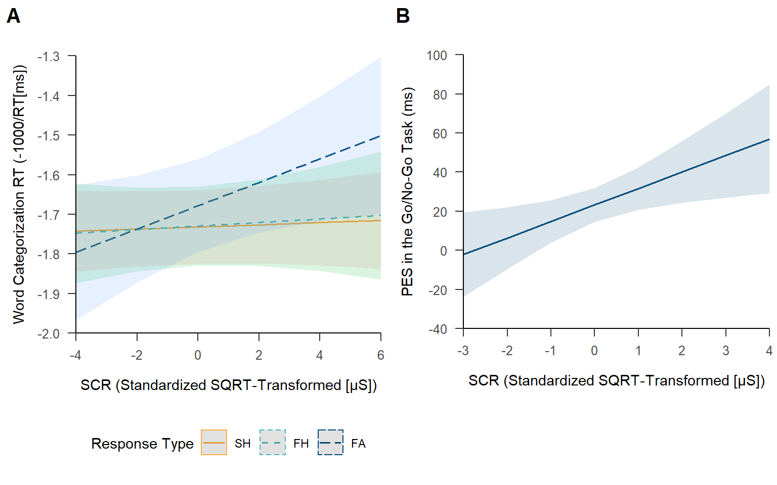
Note. (A) Estimated interaction effects of SCR and response type in the go/no-go task (SH = slow hit; FH = fast hit; FA = false alarm) on word categorization response time (RT). The slope is significant only for false alarms, indicating that following incorrect responses, an enhanced SCR is associated with slower responses to words and hence more post-error slowing. (B) Estimated effect of SCR on PES in the go/no-go task. PES was quantified using the method proposed by Dutilh et al. (2012). Shaded areas represent 95% confidence intervals. SQRT = square root.
Correlations
We calculated correlations between priming effect and SCR (for FA and FH) and between SCR and PES. PES was quantified as the error-related slowing in the subsequent go/no-go trial using the method proposed by Dutilh et al. (2012).
# Calculate individual score for priming (after FA and FH)
priming <- single_trial_data %>%
  # Apply trial exclusion criteria for priming effect
  dplyr::filter(
    word_accuracy == "correct" &
    (is.na(gng_rt_invalid)  | gng_rt_invalid  == FALSE) &
    (is.na(word_rt_outlier) | word_rt_outlier == FALSE)) %>%
  # Calculate mean per participant
  dplyr::group_by(participant_id) %>%
  dplyr::summarize(
    pos_after_FA     = mean(word_rt[gng_response_type == "FA" & word_valence == "pos"], na.rm = TRUE),
    neg_after_FA     = mean(word_rt[gng_response_type == "FA" & word_valence == "neg"], na.rm = TRUE),
    priming_after_FA = pos_after_FA - neg_after_FA,
    pos_after_FH     = mean(word_rt[gng_response_type == "FH" & word_valence == "pos"], na.rm = TRUE),
    neg_after_FH     = mean(word_rt[gng_response_type == "FH" & word_valence == "neg"], na.rm = TRUE),
    priming_after_FH = neg_after_FH - pos_after_FH) %>%
  dplyr::mutate(participant_id = factor(participant_id)) %>%
  dplyr::ungroup()


# Calculate individual score for SCR (after FA)
SCR_z_FA <- single_trial_data_scr %>%
  # Necessary to make contrast columns having same name unique
  setNames(make.unique(names(.))) %>%
  # Select only FA trials
  dplyr::filter(gng_response_type == "FA") %>%
  # Scale SCR for this data subset
  dplyr::group_by(participant_id) %>%
  dplyr::mutate(iscr_gng_resp_z_FA = scale(iscr_gng_resp, center = TRUE, scale = TRUE)) %>%
  # Calculate mean per participant
  dplyr::summarize(SCR_z_FA = mean(iscr_gng_resp_z_FA, na.rm = TRUE)) %>%
  dplyr::ungroup()


# Calculate individual score for SCR (after FH)
SCR_z_FH <- single_trial_data_scr %>%
  # Necessary to make contrast columns having same name unique
  setNames(make.unique(names(.))) %>%
  # Select only FH trials
  dplyr::filter(gng_response_type == "FH") %>%
  # Scale SCR for this data subset
  dplyr::group_by(participant_id) %>%
  dplyr::mutate(iscr_gng_resp_z_FH = scale(iscr_gng_resp, center = TRUE, scale = TRUE)) %>%
  # Calculate mean per participant
  dplyr::summarize(SCR_z_FH = mean(iscr_gng_resp_z_FH, na.rm = TRUE)) %>%
  dplyr::ungroup()


# Calculate individual score for robust PES
PES_gng <- single_trial_data %>%
  dplyr::filter(!is.na(pes)) %>%
  dplyr::group_by(participant_id) %>%
  dplyr::summarize(PES_gng = mean(pes, na.rm = TRUE)) %>%
  dplyr::mutate(participant_id = factor(participant_id)) %>%
  dplyr::ungroup()


# Create dataframe for correlations
df_correlations <- left_join(priming, SCR_z_FA,         by = "participant_id")
df_correlations <- left_join(df_correlations, SCR_z_FH, by = "participant_id")
df_correlations <- left_join(df_correlations, PES_gng,  by = "participant_id")


# Calculate correlations
corr_priming_FA_scr <- cor.test(df_correlations$priming_after_FA, df_correlations$SCR_z_FA)
corr_priming_FH_scr <- cor.test(df_correlations$priming_after_FH, df_correlations$SCR_z_FH)
corr_pes_scr        <- cor.test(df_correlations$PES_gng,          df_correlations$SCR_z_FA)


# Dispay correlations
my_table_template(rbind(cbind("Priming - SCR for FA", round(corr_priming_FA_scr$estimate, digits = 2),
                              corr_priming_FA_scr$parameter, round(corr_priming_FA_scr$p.value, digits = 3)),
                        cbind("Priming - SCR for FH", round(corr_priming_FH_scr$estimate, digits = 2),
                              corr_priming_FH_scr$parameter, round(corr_priming_FH_scr$p.value, digits = 3)),
                        cbind("PES and error-related SCR", round(corr_pes_scr$estimate, digits = 2),
                              corr_pes_scr$parameter, round(corr_pes_scr$p.value, digits = 3))),
col_names = c("", "r", "df", "p value"))| r | df | p value | |
|---|---|---|---|
| Priming - SCR for FA | -0.18 | 28 | 0.334 |
| Priming - SCR for FH | -0.28 | 28 | 0.134 |
| PES and error-related SCR | -0.01 | 28 | 0.974 |
There was no significant correlation between priming effect and SCR or between error-related SCR and PES at the between-participant level.
Control Analyses
We tested whether the SCR is affected by the valence of the word presented following the go/no-go response or by the fixation cross preceding the go/no-go stimulus and reflecting different feedback (white cross: previous response in the go/no-go task correct; red cross: previous response in the go/no-go task too slow or incorrect). Analyses were conducted using LMMs with the fixed factors response type (slow hit, fast hit, false alarm) and word valence (positive, negative) or fixation cross color (white, red), respectively. These control analyses (see below) suggested that the SCR is not confounded by events within the time window of interest.
Word valence
We did not observe any differences in SCR depending on word valence.
#### 1) Run model with maximal random-effects structure
LMM_scr_word_valence_max <- lmer(iscr_gng_resp_sqrt ~ gng_response_type * word_valence +
  (1 + FH_SH + FA_FH + pos_neg + FH_SH:pos_neg + FA_FH:pos_neg | participant_id) +
  (1 + FH_SH + FA_FH | word),
data = single_trial_data_scr,
REML = FALSE,
control = lmerControl(optimizer = "bobyqa")
)


# Check model output
summary(LMM_scr_word_valence_max) # Singular fit


#### 2) Run zero-correlation parameter model by using || syntax to reduce model complexity
LMM_scr_word_valence_red1 <- lmer(iscr_gng_resp_sqrt ~ gng_response_type * word_valence +
  (1 + FH_SH + FA_FH + pos_neg + FH_SH:pos_neg + FA_FH:pos_neg || participant_id) +
  (1 + FH_SH + FA_FH || word),
data = single_trial_data_scr,
REML = FALSE,
control = lmerControl(optimizer = "bobyqa")
)


# Check model output
summary(LMM_scr_word_valence_red1) # Singular fit


# Check PCA of random-effects variance-covariance estimates
summary(rePCA(LMM_scr_word_valence_red1)) # For participant and word stimuli there are terms that do not explain variance (< 0.5%)


# Check which random effect explains near zero variance
print(VarCorr(LMM_scr_word_valence_red1), comp = "Variance") # It is pos_neg for participant and intercept and FA_FH for word stimuli
#### 3) Run final model without random terms explaining zero variance
# (i.e., remove pos_neg for participant and intercept and FA_FH for word)
LMM_scr_word_valence_final <- lmer(iscr_gng_resp_sqrt ~ gng_response_type * word_valence +
(1 + FH_SH + FA_FH + FH_SH:pos_neg + FA_FH:pos_neg || participant_id) +
(0 + FH_SH || word),
data = single_trial_data_scr,
REML = TRUE,
control = lmerControl(optimizer = "bobyqa")
)
# Check model output
# summary(LMM_scr_word_valence_final) # Model does converge, no singular fit
# Re-check PCA of random-effects variance-covariance estimates
# summary(rePCA(LMM_scr_word_valence_final)) # All terms explain variance
# Display results (fixed effects)
tab_model(LMM_scr_word_valence_final,
dv.labels = "SCR
", pred.labels = labels, show.stat = TRUE, show.icc = FALSE, show.r2 = FALSE,
show.re.var = FALSE, show.ngroups = FALSE, string.est = "b", string.stat = "t value",
string.ci = "95 % CI", string.p = "p value", p.val = "satterthwaite"
)
# Display random effects
print("Random effects:")
print(VarCorr(LMM_scr_word_valence_final), digits = 1, comp = "Std.Dev.")| SCR | ||||
|---|---|---|---|---|
| Predictors | b | 95 % CI | t value | p value |
| Intercept | 0.42 | 0.37 – 0.47 | 15.60 | <0.001 |
| FH - SH | 0.02 | -0.00 – 0.04 | 1.74 | 0.091 |
| FA - FH | 0.10 | 0.05 – 0.16 | 3.88 | 0.001 |
| Pos - Neg | 0.00 | -0.01 – 0.02 | 0.25 | 0.803 |
| FH - SH x Pos - Neg | 0.00 | -0.03 – 0.04 | 0.28 | 0.784 |
| FA - FH x Pos - Neg | -0.02 | -0.06 – 0.03 | -0.82 | 0.417 |
| Observations | 7139 | |||
[1] "Random effects:"
 Groups           Name          Std.Dev.
 word             FH_SH         0.03
 participant_id   FA_FH:pos_neg 0.03
 participant_id.1 FH_SH:pos_neg 0.02
 participant_id.2 FA_FH         0.13
 participant_id.3 FH_SH         0.03
 participant_id.4 (Intercept)   0.14
 Residual                       0.27
Fixation cross color
# Define contrasts (sliding difference contrasts)
contrasts(single_trial_data_scr$fixation_cross_white) <- contr.sdif(2)
contrasts(single_trial_data_scr$gng_response_type)    <- contr.sdif(3)


# Add contrasts as numerical covariates via model matrix
model_matrix <- model.matrix(~ gng_response_type * fixation_cross_white, single_trial_data_scr)


# Attach the model matrix (6 columns) to the dataframe
single_trial_data_scr[, (ncol(single_trial_data_scr) + 1):(ncol(single_trial_data_scr) + 6)] <- model_matrix


# Assign descriptive names to the contrasts
names(single_trial_data_scr)[(ncol(single_trial_data_scr) - 5):ncol(single_trial_data_scr)] <- c(
  "Grand Mean", "FH_SH", "FA_FH", "red_white", "FH_SH:red_white", "FA_FH:red_white"
  )
We did not observe any differences in SCR depending on the color of the fixation cross preceding the go/no-go stimulus and reflecting different feedback.
#### 1) Run model with maximal random-effects structure
LMM_scr_cross_max <- lmer(iscr_gng_resp_sqrt ~ FH_SH + FA_FH + red_white + FH_SH:red_white + FA_FH:red_white  +
  (1 + FH_SH + FA_FH + red_white + FH_SH:red_white + FA_FH:red_white | participant_id),
data = single_trial_data_scr,
REML = FALSE,
control = lmerControl(optimizer="bobyqa")
)


# Check model output
summary(LMM_scr_cross_max) # Singular fit


#### 2) Run zero-correlation parameter model by using || syntax to reduce model complexity
LMM_scr_cross_red1 <- lmer(iscr_gng_resp_sqrt ~ FH_SH + FA_FH + red_white + FH_SH:red_white + FA_FH:red_white  +
  (1 + FH_SH + FA_FH + red_white + FH_SH:red_white + FA_FH:red_white || participant_id),
data = single_trial_data_scr,
REML = FALSE,
control = lmerControl(optimizer="bobyqa")
)


# Check model output
summary(LMM_scr_cross_red1) # Singular fit


# Check PCA of random-effects variance-covariance estimates
summary(rePCA(LMM_scr_cross_red1)) # For participant there is are terms that do not explain variance (< 0.5%)


# Check which random effect explains near zero variance
print(VarCorr(LMM_scr_cross_red1), comp = "Variance")
#### 3) Run final model without random terms explaining zero variance
LMM_scr_cross_final <- lmer(iscr_gng_resp_sqrt ~ FH_SH + FA_FH + red_white + FH_SH:red_white + FA_FH:red_white +
(1 + FH_SH + FA_FH + red_white || participant_id),
data = single_trial_data_scr,
REML = TRUE,
control = lmerControl(optimizer="bobyqa")
)
# Check model output
# summary(LMM_scr_cross_final) # Model does converge, no singular fit
# Re-check PCA of random-effects variance-covariance estimates
# summary(rePCA(LMM_scr_cross_final)) # All terms explain variance
# Display results (fixed effects)
tab_model(LMM_scr_cross_final,
dv.labels = "SCR
", pred.labels = labels, show.stat = TRUE, show.icc = FALSE, show.r2 = FALSE,
show.re.var = FALSE, show.ngroups = FALSE, string.est = "b", string.stat = "t value",
string.ci = "95 % CI", string.p = "p value", p.val = "satterthwaite"
)
# Display random effects
print("Random effects:")
print(VarCorr(LMM_scr_cross_final), digits = 1, comp = "Std.Dev.")| SCR | ||||
|---|---|---|---|---|
| Predictors | b | 95 % CI | t value | p value |
| Intercept | 0.42 | 0.37 – 0.47 | 15.52 | <0.001 |
| FH_SH | 0.01 | -0.01 – 0.03 | 1.29 | 0.205 |
| FA_FH | 0.10 | 0.05 – 0.16 | 3.89 | <0.001 |
| red_white | -0.02 | -0.04 – 0.00 | -1.91 | 0.063 |
| FH_SH:red_white | 0.00 | -0.03 – 0.03 | 0.24 | 0.813 |
| FA_FH:red_white | 0.01 | -0.04 – 0.05 | 0.39 | 0.697 |
| Observations | 7139 | |||
[1] "Random effects:"
 Groups           Name        Std.Dev.
 participant_id   (Intercept) 0.15
 participant_id.1 FH_SH       0.03
 participant_id.2 FA_FH       0.13
 participant_id.3 red_white   0.04
 Residual                     0.27
SCR in trials beginning with a red compared to those with a white fixation cross did not differ significantly.
References
Dutilh, G., van Ravenzwaaij, D., Nieuwenhuis, S., van der Maas, H. L., Forstmann, B. U., & Wagenmakers, E. J. (2012). How to measure post-error slowing: A confound and a simple solution. Journal of Mathematical Psychology, 56(3), 208-216. doi:10.1016/j.jmp.2012.04.001
Leys, C., Ley, C., Klein, O., Bernard, P., & Licata, L. (2013). Detecting outliers: Do not use standard deviation around the mean, use absolute deviation around the median. Journal of Experimental Social Psychology, 49(4), 764-766. https://doi.org/10.1016/j.jesp.2013.03.013
Morey, R. (2008). Confidence intervals from normalized data: A correction to Cousineau (2005). Tutorials in Quantitative Methods for Psychology, 4(2), 61-64. https://doi.org/10.20982/tqmp.04.2.p061
Session Info
sessionInfo()R version 3.6.1 (2019-07-05)
Platform: x86_64-w64-mingw32/x64 (64-bit)
Running under: Windows 10 x64 (build 19042)
Matrix products: default
locale:
[1] LC_COLLATE=German_Germany.1252 LC_CTYPE=German_Germany.1252
[3] LC_MONETARY=German_Germany.1252 LC_NUMERIC=C
[5] LC_TIME=German_Germany.1252
attached base packages:
[1] stats graphics grDevices datasets utils methods base
other attached packages:
[1] plyr_1.8.6 kableExtra_1.1.0 cowplot_1.0.0 sjPlot_2.8.4
[5] MASS_7.3-51.4 lmerTest_3.1-0 lme4_1.1-21 Matrix_1.2-17
[9] ggsignif_0.6.0 papaja_0.1.0.9842 ggplot2_3.3.2 knitr_1.29
[13] dplyr_0.8.3
loaded via a namespace (and not attached):
[1] httr_1.4.1 tidyr_1.0.0 viridisLite_0.3.0
[4] splines_3.6.1 modelr_0.1.5 assertthat_0.2.1
[7] highr_0.8 renv_0.12.0 yaml_2.2.0
[10] bayestestR_0.7.2 numDeriv_2016.8-1.1 pillar_1.4.6
[13] backports_1.1.5 lattice_0.20-38 glue_1.3.1
[16] digest_0.6.22 RColorBrewer_1.1-2 rvest_0.3.6
[19] minqa_1.2.4 colorspace_1.4-1 htmltools_0.4.0
[22] pkgconfig_2.0.3 broom_0.5.2 haven_2.2.0
[25] purrr_0.3.3 xtable_1.8-4 mvtnorm_1.0-11
[28] scales_1.1.0 webshot_0.5.1 emmeans_1.4.2
[31] tibble_3.0.4 generics_0.0.2 farver_2.0.1
[34] sjlabelled_1.1.3 ellipsis_0.3.0 withr_2.1.2
[37] magrittr_1.5 crayon_1.3.4 effectsize_0.3.2
[40] estimability_1.3 evaluate_0.14 nlme_3.1-140
[43] forcats_0.4.0 xml2_1.2.2 tools_3.6.1
[46] hms_0.5.2 lifecycle_0.2.0 stringr_1.4.0
[49] munsell_0.5.0 ggeffects_0.15.1 compiler_3.6.1
[52] rlang_0.4.8 grid_3.6.1 nloptr_1.2.1
[55] parameters_0.8.2 rstudioapi_0.10 labeling_0.3
[58] rmarkdown_1.16 boot_1.3-22 gtable_0.3.0
[61] codetools_0.2-16 sjstats_0.17.8 sjmisc_2.8.2
[64] R6_2.4.1 performance_0.4.3 insight_0.9.0
[67] readr_1.3.1 stringi_1.4.3 Rcpp_1.0.5
[70] vctrs_0.3.4 tidyselect_0.2.5 xfun_0.16